cauer.mws
syntfil[Cauer]
- compute the Cauer approximation
syntfil[CauerB]
- compute the type B Cauer approximation
syntfil[CauerC]
- compute the type C Cauer approximation
Calling sequence:
Cauer(order, Os, ap, var)
CauerB(order, Os, ap, var)
CauerC(order, Os, ap, var)
Parameters:
order -
order of the Cauer approximation [-]
Os -
stopband frequency of normalized lowpass (NLP) [1/s]
ap -
passband ripple [dB]
var -
variable symbol in tranfer and characteristic function
Parameter
order
must be positive integer and for type B and C in addition even. Parameters
Os
and
ap
must be positive numbers where
Os
>
1
. Parameter
var
must be
symbol
.
Description:
-
This function returns inverse transfer function
 , characteristic function
 and one dimensional array of transfer function's zeros.
-
Inverse transfer function is rational function with polynomial in numerator and denominator in variable
var
. Numerator polynomial has degree
order
. Denominator polynomial has degree
order
for even order or
order-1
for odd order. In case of type B and C the denominator polynomial has degree
order-2
.
-
Characteristic function is also rational function. Denominator of
 is identical with denominator of
 . Zeros and poles of
 lay on imaginary axis.
-
Cauer approximation of type B is computed from standard Cauer aproximation (type A), which in case of even order eventuates to negative element value (L or C) at realization of LC ladder filter.
-
Cauer approximation of type C is computed from Cauer aproximation of type B.
-
Info level:
Setting of variable
infolevel[syntfil]
can be used to get more detailed results.
infolevel[syntfil] =
2 -
print polynomials of inverse transfer function characteristic function and zeros of transfer function on separate lines with description.
3 -
as level 2 +
print transfer function's poles and parameter
 .
.
4 -
as level 3 +
print characteristic function's poles and zeros.
5 -
for type B -
as level
4 + print transfer and characteristic function's poles and zeros for type A,
-
for type C -
as level
4 + print transfer and characteristic function's poles and zeros for type A and B.
Example:

![`You can set infolevel[syntfil] variable to 2..5 to get more detailed results!`](images/cauer9.gif)
Type A Cauer approximation
| > |
G_a,Phi_a,zeros_a:=Cauer(4,1.2,3,s);
|


Type B and C Cauer approximation
| > |
G_b,Phi_b,zeros_b:=CauerB(4,1.2,3,s);
|
| > |
G_c,Phi_c,zeros_c:=CauerC(4,1.2,3,s);
|

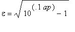
epsilon = .9976283451
Poles of H:
[-.3962720440+.3402416437*I, -.3962720440-.3402416437*I, -.7308417727e-1+.9606838030*I, -.7308417727e-1-.9606838030*I]
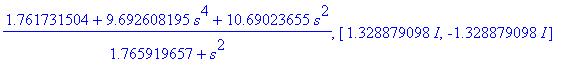
CauerC:
G = (1.959408974+7.737846293*s^4+7.263612593*s^3+10.18993450*s^2+6.001139906*s)/(1.959408973+s^2)
Phi = (7.737846293*s^4+6.780712709*s^2)/(1.959408973+s^2)
Zeros = [1.399788903*I, -1.399788903*I]


Magnitude frequency response for type
A
,
B
a
C.
| > |
plot([MagnitudeHdB(1/G_a)(omega),MagnitudeHdB(1/G_b)(omega),MagnitudeHdB(1/G_c)(omega)],omega=0..5,-60..0,color=[red,green,blue]);
|
![[Maple Plot]](images/cauer16.gif)
See also:
CauerNLPOrder
CauerPolesZeros,
CauerBOmega,
Cauer_asnew
DroppNLP,
TestCharEqn,
sortzeros,
MagnitudeH,
MagnitudeHdB,
PhaseH,
GroupDelayH,
in addition to Cauer approximation the following approximations can be used
Butterworth,
Chebyshev,
InvChebyschev,
InvChebyshevB